Predicting Short Radio Paths with Radio Mobile Roger Coude' VE2DBE hosts a website called Radio Mobile. It is a fantastic resource for predicting radio paths. While it appears to me that it was best indended to predict the coverage for a radio station (think Broadcast FM), and it includes several features that add value to that intent (such as 'number of people covered'), when building a packet network it comes in handy for predicting radio paths, especially in the VHF/UHF range which, by their nature, tend to cover 'short' distances. Here, N2IRZ writes some basic instructions on what Radio Mobile can do, how to use it, and understanding the results. Much Fun Thereby!

Predicting short radio paths on VHF and UHF using Radio Mobile

Don Rotolo N2IRZ - January 2026

I play packet a lot, building and promoting a TARPN network here in Atlanta, so when someone asks how to join the network, it’s helpful to have a tool to predict relatively short RF path performance. Radio Mobile, an online tool by Roger Coude’ VE2DBE, makes this easy and delivers reliable accuracy.

Start by requesting a (free) account at his web site (for English – there’s also French, Spanish and Italian). When I asked for an account over a decade ago, I remember it took a few days for approval, but I have no recent experience. These is also an offline version you can download, but it’s a bit complicated to get it running like that. Look into it if you’re interested.

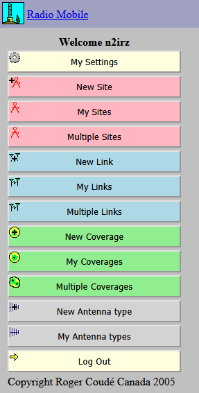
On the page mentioned above, click on the Radio Mobile Online link, where you can log in or request a new account. After login, you’ll see the Main Menu, which looks like this:

• My Settings is where you set the desired defaults for the account, as well as change the password or delete the account. The choices are mostly self-explanatory, but we’ll take a closer look at this in a moment.
• Sites: New site allows you to define a site, the first step in any link or coverage study. Once defined, it will appear in My Sites. You can select several sites using Multiple Sites and show them all on a single map.
• Links: New Link defines a link between two sites, after which it can be saved to My Links. Multiple Links allows you to show several links on a single map.
• Coverage: You can probably guess this, but New Coverage defines a new site coverage plot, which can be saved to My Coverages, and Multiple Coverages can all be shown on a single map.
• Antennas: Pre-defining antenna types can be useful, but I tend to use either a default omnidirectional antenna or a known-gain Yagi. Antennas can also be saved.
• Log Out is just what it says.

First, let’s step through defining a new site.

When you click the "new Site" button, you’ll see a map of Earth with a cursor centered in the Atlantic Ocean at 0 00’ 00”, 0 00’ 00”. Drag the map so your home location is kind of near the center of the display (within a few hundred miles is fine), then zoom in (zoom controls are at the upper left, or a scroll wheel mouse also zooms) while re-centering, repeating that until you’ve zoomed in quite a lot and see individual buildings and roads, and your antenna’s location is near the center of the display. Click the “Place cursor at center” button at the bottom, then adjust the exact position of the ‘center’ and click again until the cursor is located exactly where your antenna is. NOTE: Don’t click “Center at Cursor” as that will bring you right back to 0,0 in the Atlantic! Don’t ask how long it took to break myself of that unfortunate habit…

Then click Submit, which brings up the New Site Dialog.

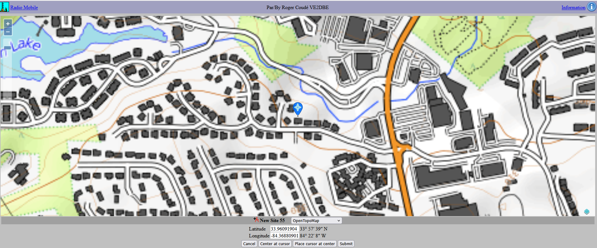
In the new site dialog, you can adjust the exact latitude and longitude, give it a name (definitely do this!) and assign a description (like N2IRZ Home Atlanta) and designate a group (like TARPN Sites). Once you’re satisfied, click “Add to My Sites to save it. You’ll need to do this for each and every antenna site you want to work with.

Once saved, you’ll be returned to the main menu.

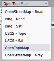
Let’s define another site, using the same process. Pick something a few miles away, exactly where isn’t important now, but of course it can be a real site you’ll want if you like. Once you have the cursor in the right place, but before you Submit it, try each of the available map options:

My personal preference is Open Topo Map, with Open Street Map my second choice. Both show building locations, which is handy (although not always 100% accurate). Be patient if you pick some of the maps, as they may need some time (could be several minutes!) to populate.

Once you have found a favorite, and you’ve completed defining this second site, set the default map type in My Settings.

OK, now that we have two sites defined, let’s try a few things.

1. FIRST: Click on My Sites, where you can perform several actions on the site record, particularly these three things:

   • Modify: Change any aspect of the site record.
   • Define as Home in my settings: Definitely do this, for if you do not the New Site cursor will always start back in the Atlantic Ocean. In general, your home site will be closer to your areas of interest than 0,0 would be, making new site definition a bit simpler.
   • Export to (and Import from) CSV: This allows you to generate a Comma Separated Values file, easily editable using a text processor, Microsoft Excel or any other program that handles the common CSV format. I prefer Excel. We’ll look at this in detail later.

   Also note that at the very top, you can pick any of the defined sites.

   Click Return to main menu

2. SECOND: Click Multiple Sites. In the dialog that opens, pick both of your sites.

   Clicking selects one site, Shift-Click lets you select several sites next to each other on the list, and Ctrl-Click lets you select several sites with some not selected on the list. This makes more sense when there are several defined sites. Also note you can filter sites by text.

   Then click Submit. A map showing the selected site(s) is shown, and you can pan, zoom and otherwise manipulate the display. You can also change map type.

   This feature is really handy when you want to show the physical location of several sites relative to each other and geographic features such as roads and lakes. The only unfortunate thing with this feature is that name/callsign and (more or less) exact locations are shown, which might cause some privacy concerns, so use discretion and ask your contacts for permission. Use Return to Multiple Sites and Return to Main menu.

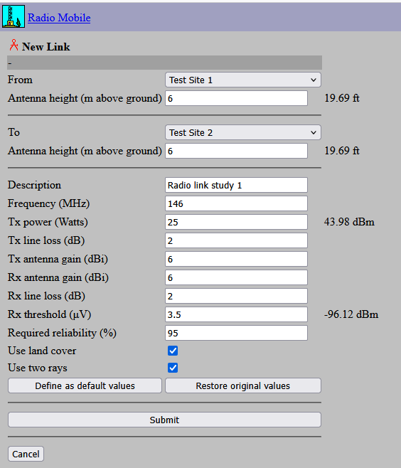
3. THIRD: Define a link. Click on New Link, which opens the new link dialog. Here you have several important settings to deal with, and their accuracy will directly impact the accuracy of your link study.

   The Radio Mobile defaults should be modified to the values shown on the next page. We’ve spent some time and effort to develop these particular values, so please use them until you find that your predictions are either overly optimistic or pessimistic, after which you should develop your own, new, default

These new defaults are very conservative, so if this shows your link will work, it’s certain that it will. Here are the specific settings, which we’ll discuss in a moment:

• Antenna height above ground should be set to 6 meters (about 20 ft) for both stations.
• Set the frequency to one of the bands you’ll often use, such as 146 MHz.
• Set the TX power to a value you’ll commonly use, such as 25W
• TX (and RX) line loss should be 2 dB.
• TX (and RX) antenna gain should be 6 dBi.
• RX Threshold should be set to 3.5 uV.
• Required reliability should be 95%.
• Both checkboxes should be checked.

Then click “Define as default values”

So, what do all these things mean?

• Antenna Height: Starting at 6 meters is good, because almost everyone can get an antenna up 20 feet in the air. If you know that the antenna can go higher, then set it to its actual height. This value has a large influence on the calculated path loss, which is the most important number we will use to decide if the path will work or not. More on that soon.
• Frequency should use the actual frequency, or close to it, because that also affects calculated path loss. Lower frequencies propagate better. You’d see a difference between 146 MHz and 144.91 MHz.
• TX Power is almost irrelevant, as are the rest of the settings. The reason is that once we know the calculated path loss (a function of antenna height, frequency, and terrain), we know what kind of signal we have to throw at the link to overcome it.
  More signal (a combination of TX power, antenna gain, reduced feedline loss) can overcome a given path loss, but you’ll find that a path loss above a certain value (about 152 dB) becomes prohibitive. Most land-mobile commercial radios I use for packet have 25W output, some have more, some have less. If you use the correct value, this makes the prediction that it will (or won’t) work more accurate, but it doesn’t affect the path loss at all.
• TX and RX line loss is a function of cable type, frequency and length. For example, 100 feet of LMR400 has 1.5 dB loss at 150 MHz and 2.7 dB at 450 MHz. 2 dB is a reasonable number, factoring in losses from connectors and such. You can fool yourself by making this 1 or 0, but a dB or two is just a rounding error here. Leave it at 2.
• Antenna gain is another way to fool yourself into thinking a path will work. An X50 omnidirectional antenna has 4.5 dB gain on 145 MHz and 7.2 dB on 430 MHz, but note these values are dBi (which is what Radio Mobile needs) and not dBd, which is used by some manufacturers. dBd gain is about 2.1 dB lower than dBi, or in other words 0 dBd is 2.1 dBi. If dBi and dBd are not clear to you, the internet can advise you what this means.
• Rx threshold (uV) is the voltage at the radio antenna’s terminals needed for a ‘good’ signal. This translates to -96.12 dBm, which is typically sufficient for a 20 dB receiver SINAD noise level, and may be a bit conservative. You can fiddle with this if you fully understand what this means and have the receiver’s specs, but you can also fool yourself, so beware.
• Required reliability is how often the signal will be above the value needed to be ‘good’. The original default of 70% would be fine for listening to an FM broadcast station like 102.7, but packet is more demanding. We’ve found empirically that 95% is a good value.

Below is the result for my test link, which has three sections:

• Top, showing the path form the side, including terrain
• Center, with all the calculated and defined values
• Bottom, a map of the link superimposed on a map

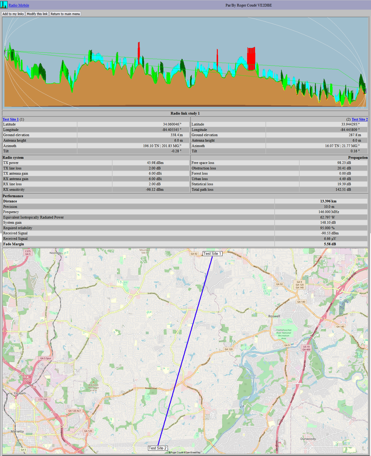
At the very top, three buttons allow you to add the link to your list of links, modify the link, or return to the main menu. Once you have the link set up how you want it – you can modify it indefinitely – I strongly recommend you select Modify one last time and give the link a name (in the Description field) like “Don – Bob 2m 25W 10dB” (meaning a link between Don and Bob (use callsigns if preferred), on 2 meters, using 25 Watts, with 10 dBi antennas). Once you get a dozen or more links, it’s nice to know which one is which.

In the top section, note the following: The two antennas are at the extreme left and right sides of the image. Between them, we see the rise and fall of the Earth, along with four colors, whose exact meaning I have not yet figured out, but I can see that red is bad and green is good. (If you find info on this, please let me know!).

If you think of Radio Mobile as a tool used to show the coverage of a broadcast station (think TV station), then I speculate that these colors show the places along a certain path where a certain level of reception can occur, or not.

You can also see reception lines – her seen as two green lines, but if you have direct line of sight it will show only one line. Yellow lines mean a marking path, red lines mean no path.

In the bottom section, we see the path on a map. In the download/offline version, it says that clicking in the top section (say, on a hilltop) puts a marker on the bottom section map, helping identify a hill that’s causing your troubles. This doesn’t work in the online version.

Then there’s the middle section, in which we are most interested.

We see the details of Test Site 1 (and Test Site 2): lat/lon, altitude, antenna height, azimuth (the compass direction from this station to the other station (in True North as you’d find on a map, and Magnetic North as your cell phone’s compass will display, handy for pointing a yagi)), and antenna tilt (how far the other station is above or beneath this one – ignore values less than a few degrees).

The Radio System is described: These are the things you can change to increase the overall system gain, but if these don’t match reality you can be fooling yourself. Sure, set the antenna gains to 100 dBi and see what happens, but it doesn’t help if it’s not real. On the other hand, carefully adjusting these values can help you understand what might be needed to make a path work: Upgrade an antenna by 3 or 6 dB, double power (adding 3 dB), etc.

Propagation provides the calculations that show whether the path can be made to work or not. The various calculated losses are specified, ending with a Total Path Loss. Values over about 152 dB are typically impractical. Values in the lower 140s are good, in the 130s great and below that excellent. You can affect this number by adjusting the antenna height(s) and radio frequency. Lower frequencies go further, so if a 440 MHz path comes in with a total path loss of 156 dB you might find that it drops to 147 dB at 145 MHz.

In this specific example, if we raise the Test Site 2 antenna to 10 meters (33 ft) from 6 meters, you clear that small hill right near test Site 2 and change the path loss to 137.15 dB from 142.51 dB, an improvement of 5.36 dB, which is significant. Raising the Test Site 1 antenna has little effect, as the nearby terrain is already being cleared.

With Test Site 2’s antenna at 10 meters, if we then change frequency to 440 MHz, the path loss becomes 147.73 dB from 137.15 dB, a very significant degradation, although antenna gain is less expensive on the higher frequencies. If we split the difference and use 223 MHz, the 140.88 dB path loss is actually not too bad. This link doesn’t require 145 MHz, 223 MHz will do just fine.

Lastly, we see Performance. This shows us the values calculated and what we might expect for received signal and fade margin (compared to the required 3.5 uV signal for 95% reliability). Again, we can fool ourselves if we’re not careful, but this section can also give clues as to where to put out efforts for a better link. If we’re using real numbers, a fade margin for a good link should exceed 10 dB, higher being better. This accounts for things like attenuation from rain, snow, wet foliage and the like.

Link calculations are a great way to identify which of several options might offer best performance. For example, I have three neighbors, David, Bob and Jon.

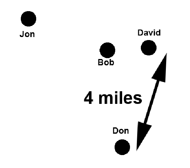
I can reach any one of them on 2 meters, but David has the lowest Total Path Loss (TPL), and 223 still offers an excellent path with 129.59 dB TPL. If necessary, I could use 440 MHz if necessary, but I already have a 440 link to Brian (not shown), a minor dilemma.

David can reach Bob, but TPL on 440 is over 156 dB (even though they are only a mile apart, there’s a big hill in the way), David already has 223 MHz on the air (from me), so on 145 MHz the TPL is 132.87 dB, which is excellent.

Bob can reach me on 145 MHz, with 138.24 dB TPL, but then he’d be unable to reach David directly. Bob can reach Jon on 223 MHz with 136.19 dB TPL, again quite good. 440 between Bob and Jon has 143.38 dB TPL, not bad but we can do better.

Lastly, Jon can reach me on 145 MHz with 136.28 dB TPL.

The resulting ‘ideal’ network would look like this. We have a loop, meaning that any one link can fail yet all stations would retain connectivity, and if one node failed, then the other nodes would stay connected.

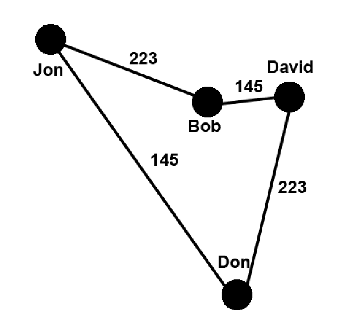
For this example, I had to model 5 links on each of three bands to identify the best options. Some were obvious, but some were judgement calls. It does help that we have radios for all three common amateur bands.

The last menu section is Coverage. As with other sections, we can define a new coverage, manage a list of existing coverages, and show multiple coverages on a single map. Exporting the coverage data (available in several file formats, including .png and .kml) allows one to use a graphics program or Google Earth (the local version, not online) to display coverages in useful ways.

As mentioned previously, I get the impression that the coverages ‘module’ is more meant for something like TV or FM radio station coverage than for ham radio path predictions, but it serves a useful purpose nonetheless.

This image shows the default values I use for coverages. Many of these values are the same as for link calculations (however note the antenna settings at top. I use Omni as a default, but in some cases Yagi might be appropriate), but near the bottom we have a few new choices:

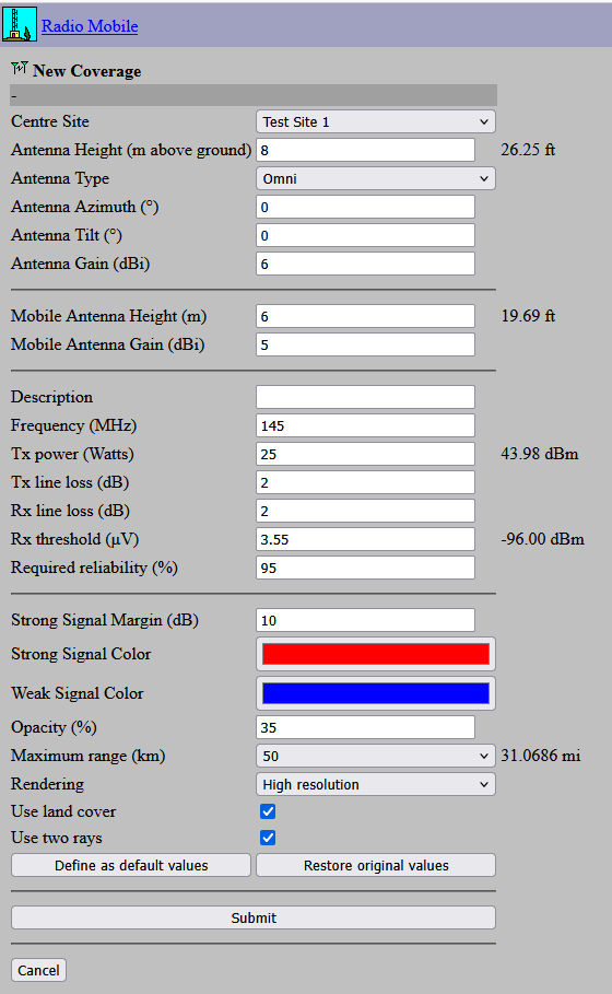
Strong signal margin: This is where the color changes from Strong to Weak.

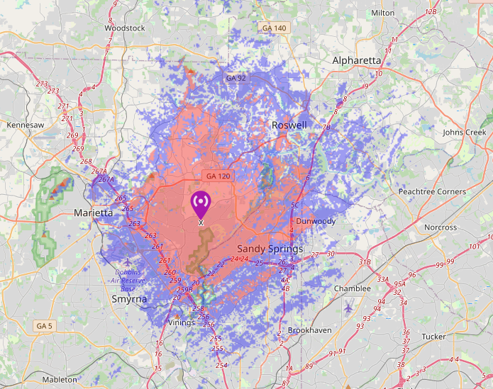
Signal Color(s): How coverage is shown, both strong and weak. You can set most any colors here, but I’ve found that these colors (red and blue) show up best on maps. All coverage plots should use the same colors, because when you try to view Multiple Coverages, too many colors gets very confusing.

Opacity (%) is how opaque the colors are against the map. 35% is good.

Maximum range (km) is the diameter of the circle around the station that coverage is calculated in. On hilly terrain, 50 km may be too far, while in flat terrain too close. Higher numbers dramatically increase the calculation time. In hilly North Atlanta, 50 km is a bit large but reasonable, as I rarely hit the edge of the circle.

Rendering can be Low, High and Very High resolution. This setting has a HUGE impact on calculation time: a 50 km circle on Low takes a minute or two, on High maybe 2 or 3 minutes, and on Very High up to 5 minutes. I’ve found High (1001x1001 pixels) is plenty, but you should play with these. Your computer isn’t doing the calculations, the web server is, so upgrading your CPU or GPU won’t affect much here.

When you’re happy, set the default. Beware of accidentally clicking Restore Original Values, as this erases everything.

To get the coverage plot, click Submit. Here is an example from the data used above. You have a few choices of map background as well. We can see that reaching Woodstock (upper left) and Alpharetta (upper right) are unlikely but much of Western Sandy Springs offers solid coverage. Some coverage can also be expected in Roswell, but it varies widely.

I’m not going to get into the details of downloading coverage data (it must first be saved to “My Coverages”) but if you know what a .kml file is you’ll be able to figure it out.

One last thing about Multiple Coverages: A hypothetical example. Bob (in Kennesaw) and Dom (in Villa Rica) wanted to build a link, but they were too far apart even for 145 MHz. We put up both their coverage plots on the same map, and they overlapped in the town of Dallas. Someone cold-called Ethan (we’d looked up all the hams in that area using < https://haminfo.tetranz. com/map> and found his contact info on QRZ.com), and he was interested (much to our surprise), so we had dinner and, long story short, built two links to connect Bob to Don through Ethan.

While this quick intro is intended to steer you when using Radio Mobile, the best action is for you to actually do things yourself, make mistakes (and learn from them), and become your own expert. I’ve found great results on VHF/UHF, but Radio Mobile can be used on most any amateur frequency. I can’t say how well it’ll predict propagation on 40 meters, since I’m not aware that it used any atmospheric modeling, but you should go play with it and let the rest of us know what you found.

73 de N2IRZ